


Reliability of System Configurations: Statistics and Probability Questions Answers

Answer
Section A
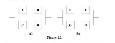
Que 1 a)
System 1.1 a)
Table given below shows all possible states of the system. IS_OPERATIONAL columns indicates whether system will be operational or not.
Probability of system being operational =
(0.2)^2*(0.8)^2 +
(0.2)*(0.8)^3 +
(0.2)*(0.8)^3 +
(0.2)^2*(0.8)^2 +
(0.2)*(0.8)^3 +
(0.2)*(0.8)^3 +
(0.8)^4
= 0.8704
System 1.1 b)
Here I am assuming an column works if at least one component of the column is operational (Please let me know if this assumption is wrong as we need to know about this but its not mentioned in the problem clearly).
Table given below shows all possible states of the system. IS_OPERATIONAL columns indicates whether system will be operational or not.
Probability of system being operational =
(0.2)^2*(0.8)^2 +
(0.2)^2*(0.8)^2 +
(0.2)*(0.8)^3 +
(0.2)^2*(0.8)^2 +
(0.2)*(0.8)^3 +
(0.2)*(0.8)^3 +
(0.2)*(0.8)^3 +
(0.2)^2*(0.8)^2 +
(0.8)^4
=0.9216
So, probability of system in 1.1 b) to be operational is higher than system in 1.1 a). So system in 1.1 b) is more reliable.
System 1.1 a)
| index | A | B | C | D | IS_OPERATIONAL |
| 0 | 0 | 0 | 0 | 0 | NO |
| 1 | 0 | 0 | 0 | 1 | NO |
| 2 | 0 | 0 | 1 | 0 | NO |
| 3 | 0 | 0 | 1 | 1 | YES |
| 4 | 0 | 1 | 0 | 0 | NO |
| 5 | 0 | 1 | 0 | 1 | NO |
| 6 | 0 | 1 | 1 | 0 | NO |
| 7 | 0 | 1 | 1 | 1 | YES |
| 8 | 1 | 0 | 0 | 0 | NO |
| 9 | 1 | 0 | 0 | 1 | NO |
| 10 | 1 | 0 | 1 | 0 | NO |
| 11 | 1 | 0 | 1 | 1 | YES |
| 12 | 1 | 1 | 0 | 0 | YES |
| 13 | 1 | 1 | 0 | 1 | YES |
| 14 | 1 | 1 | 1 | 0 | YES |
| 15 | 1 | 1 | 1 | 1 | YES |
System 1.1 b)
| index | E | F | G | H | IS_OPERATIONAL |
| 0 | 0 | 0 | 0 | 0 | NO |
| 1 | 0 | 0 | 0 | 1 | NO |
| 2 | 0 | 0 | 1 | 0 | NO |
| 3 | 0 | 0 | 1 | 1 | YES |
| 4 | 0 | 1 | 0 | 0 | NO |
| 5 | 0 | 1 | 0 | 1 | NO |
| 6 | 0 | 1 | 1 | 0 | YES |
| 7 | 0 | 1 | 1 | 1 | YES |
| 8 | 1 | 0 | 0 | 0 | NO |
| 9 | 1 | 0 | 0 | 1 | YES |
| 10 | 1 | 0 | 1 | 0 | NO |
| 11 | 1 | 0 | 1 | 1 | YES |
| 12 | 1 | 1 | 0 | 0 | YES |
| 13 | 1 | 1 | 0 | 1 | YES |
| 14 | 1 | 1 | 1 | 0 | YES |
| 15 | 1 | 1 | 1 | 1 | YES |
Que 1 b)
Case 1: Lily starts first
Pr(‘Lily drawing cross marked paper in first trial’) = 1/x+1
Pr(‘Lily drawing cross marked paper in second trial’) = x/x+1∗x-1/x∗1/x-1= 1/x+1
Pr(‘Lily drawing cross marked paper in third trial’) = x/x+1∗x-1/x∗x-2/x-1∗x-3/x-2∗1/x-3= 1/x+1
Case 2: Lily starts second
Pr(‘Lily drawing cross marked paper in first trial’) = x/x+1∗1/x= 1/x+1
Pr(‘Lily drawing cross marked paper in second trial’) = x/x+1∗x-1/x∗1/x-2/x-1∗1/x-2= 1/x+1
Pr(‘Lily drawing cross marked paper in third trial’) = x/x+1∗x-1/x∗x-2/x-1∗x-3/x-2∗x-4/x-3∗1/x-4= 1/x+1
We can see that probability of drawing crossed paper is always equal to independent of who starts drawing the paper first. So I would recommend Lily to ask James to start to draw the paper, this will lead to James taking the risk first.
Que 2
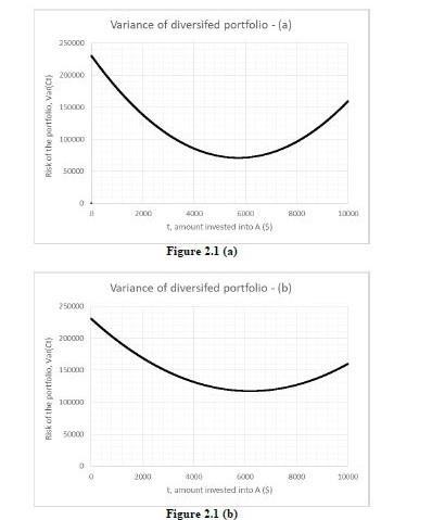
Part a)
Plot on part a looks to have lesser risk of the portfolio. Because at any value of t, the risk of the portfolio is lower in plot a as compared to plot b. One more way to explain it is the area under the curve is equal to risk of the portfolio, and it is lower for plot a.
Part b)
- Probability that the reaction time is between 0.8 sec and 1.8 sec = cdf(1.8) – cdf(0.8) = 0.9678 – 0.2578 = 0.71
- If point value k that has the property that 5% of all drivers have a reaction time of this value or lower,
then cdf(k) = 0.05
Solving for k, we will get k = 0.402
- Section B
Que 3 Data preparation task done
Que 4
KPL vs Fuel capacity
KPL vs Weight
With the limited number of sample points, we can see that there is linear association between KPL-Fuel Capacity and KPL-Weight variables.
The strength of linearity between KPL-Fuel Capacity looks higher than KPL-Weight.
Que 5
| |
|
There is negative correlation between both the pairs. The Magnitude of correlation between KPL-Fuel Capacity is higher than KPL-Weight, this verifies our guess in Question 4.
Que 6
- a) Fitted regression line
KPL = (-0.003192392)Weight + 21.54142512
- b) Interpretation
The linear regression equation above says that for every 1 unit change in weight, there is a constant decrement of 0.003192392 in KPL.
- c) This model is significant at 5% significance level. P-value of coefficient of weight is 0.031 and P-value of intercept is much lesser than 0.01.
- d) Co-efficient of determination also known as R-square statistic for the model is = 0.07694. Value of R-square statistic ranges from 0 to 1. Higher the value of R-square better is the predictive power of the model. So for our current model R-square is now very good.
- e) When we fit linear regression line, our objective function to be optimised is squared differences of actual Y value and predicted Y value. That is why linear regression is also called as least square regression line.
- f)
KPL = (-0.003192392)Weight + 21.54142512
Lower value of coefficient of weight at 95% significance level = -0.0060986
Lower value of intercept at 95% significance level = 16.2962836
Upper value of coefficient of weight at 95% significance level = -0.0002862
Upper value of intercept at 95% significance level = 26.7865666
So, 95% confidence interval of KPL =
[-0.0060986*2560 +16.2962836 , -0.0002862*2560 + 26.7865666]
= [0.6838675999999992, 26.0538946]
Interpretation of this 95% confidence interval is that if we randomly change the training data, then 95% of the times, KPL for a car with weight 2560kg will lie between [0.6838675999999992, 26.0538946]
Que 7
To determine if average value of KPL for sedan is statistically equal to average value of KPL of hatchback, we will do unpaired t-test.
H0: Average value of KPL for sedan is statistically equal to average value of KPL of hatchback
Ha: Average value of KPL for sedan is statistically not equal to average value of KPL of hatchback
If the p-value of t-test < 0.05 we reject H0 and accept Ha. But if the p-value of t-test is > 0.05 then we accept H0.
In our case p-value = 0.0005, so we reject H0.
So, average value of KPL for sedan is statistically not equal to average value of KPL of hatchback.

Customer Testimonials