Questions on Introduction to Biostatistics 2020 Assessment 3 Answer

Introduction to Biostatistics 2020

Assignment 3

[5 questions in total]

This assignment is worth 30% of the total credit for this course. [There is a total of 40 marks in this assignment, which will be rescaled in the final course mark calculations.]

Answer all questions. You may use a computer or calculator to assist with summarising data and doing intermediate calculations, but you may lose points if your answer is incorrect and you have not provided evidence of your working.

Question 1 [5 marks; 1 mark for each]

We will start with some more practise in looking up tables. State the following probability values – either exact values or the range of possible values indicated on the Statistical Tables. For each part, include a diagram to indicate the area of interest in the relevant distribution.

(a) P(t > 2.31) (for the t distribution on 18 degrees of freedom)

(b) P(t > -1.8727) (for t on 5 df)

P(c2 > 6.68) (arising from a test of association on a 2x2 contingency table)
P(c2 > 9.50) (arising from a test of association on a 4x3 contingency table)

Question 2 [7 marks]

This question concerns a study that was introduced in Assignment 2.

In a study concerning the effectiveness of Ginkgo biloba in treating tinnitus, 24 participants were recruited through advertisements in the national press in the United Kingdom. Once enrolled in the study, participants were asked to complete a number of questionnaires that allowed for the calculation of a severity of tinnitus score. Participants were then instructed to take three tablets a day (each containing 50mg of Ginkgo biloba) over a 12 week period. After this time participants completed the same questionnaires so that their severity of tinnitus could again be calculated. All participants are assumed to have complied with the treatment regimen.

If the mean severity of tinnitus score for patients at entry to the study was found to be 30.07 units (with a standard deviation of 6.10 units) and after the 12 week period was found to be 27.26 units (with a standard deviation of 5.20 units), using a Type 1 error level of 0.05 (i.e. a = 0.05), determine if there is a “statistically significant” difference in mean score before and after treatment. State the appropriate null and alternative hypotheses, and show all working. [5 marks][Note: if needed, the standard deviation of the differences (score at entry to study – score after treatment) was 7.10 units.]
State and justify your conclusion clearly so that an individual without your statistical knowledgecould understand the results.

Remember to show your working and justify your conclusions.

Question 3 [8 marks]

This question also concerns a study that was introduced in Assignment 2.

An article by Holland et al “Does home based medication review keep older people out of hospital?” (British Medical Journal 2005; doi:10.1136) concerned the reporting of evidence obtained through a randomised controlled trial intended to investigate this question. Participants were all patients aged over 80 who had experienced an emergency admission to hospital (for any cause), were prescribed two or more drugs on discharge and were returning to their own home or warden controlled accommodation.

Participants were randomised to receive either:

Intervention: two home visits by a pharmacist within two weeks and eight weeks of discharge to educate and aid patients with their medications, or

Control: standard care.

Analysis focused on 415 individuals randomised to the intervention and 414 individuals randomised to control. The primary outcome measure was the number of emergency re-admissions to hospital at 6 months.

The average number of re-admissions was 0.56 (SD = 0.87) for participants randomised to the intervention and 0.43 (SD = 0.73) for participants randomised to control.

Assuming the number of re-admissions is a continuous variable, test for a difference in (population) average number of re-admissions for participants randomised to the intervention and (population) average number of re-admissions for participants randomised to the control. Use a two-tailed test and assume a Type 1 error level of 0.05 (i.e. a = 0.05) was pre-set as acceptable.Show your working. [5 marks]
State your conclusion clearly so that an individual without your statistical knowledge could understand the results. [2 marks]
Without any calculations, briefly explain how the results of a test of a one-tailed alternative hypothesis might differ from those found in (a). [1 marks]

Questions 4 [12 marks]

In a study by Radelet and Pierce (1991), the relationship between defendant’s ethnicity and sentencing to the death penalty over a 12 year period was investigated among 674 defendants convicted of murder in Florida. Only defendants and victims who were Caucasian or African-American were considered in the study results described in this question.

a. Of the 483 Caucasian defendants, 53 were sentenced to the death penalty. Of the 191 African- American defendants, 15 were sentenced to the death penalty.

State an appropriate null and alternative hypothesis for this study. Draw a suitable 2x2 contingency table to display these data and test at the 0.05 level (i.e. a = 0.05) for an association between defendant’s ethnicity and sentencing to the death penalty. Show your working, and present your conclusion with respect to your study hypotheses. [3 marks]

Radelet and Pierce also presented information concerning the ethnicity of the murder victim.

b. There was a total of 515 Caucasian murder victims. Among the Caucasian victims, 467 defendants were also Caucasian. In these cases, there was a death penalty sentence for 53 defendants. The court determined that a total of 48 Caucasian victims were murdered by African-American defendants, and 11 of these defendants were sentenced to the death penalty.

State an appropriate null and alternative hypothesis for this component of the study concerned with C aucasian victims, clearly stating the population of interest. Create a suitable 2x2 table to display these data and test at the 0.05 level (i.e. a = 0.05) for an association between defendant’s ethnicity and sentencing to the death penalty. Show your working, and present your conclusion with respect to your study hypotheses. [3 marks]

c. There was a total of 159 African-American victims. Among the African-American victims, 16 of the convictions were for Caucasian defendants, and no death penalties were sentenced for these defendants. Both defendant and victim were African-American for 143 convictions, and the death penalty was sentenced in 4 of these murders.

State an appropriate null and alternative hypothesis for this component of the study concerned with African- American victims, clearly stating the population of interest. Create a suitable 2x2 table to display these data and test at the 0.05 level (i.e. a = 0.05) for an association between defendant’s ethnicity and sentencing to the death penalty. Show your working, and present your conclusion with respect to your study hypotheses.

d. Comment on your conclusions across parts (a) – (c).

Question 5 [8 marks]

Metatarsus adductus (MA) is a foot condition wherein the front part of the foot turns in. It is a common condition in adolescents, and usually corrects itself. Hallux abducto valgus (HAV) is a deformation of the big toe that is not usually severe in adolescents, but if severe it usually requires surgery. The severity of each of these foot conditions is measured as the angle of deformity, where higher angles indicate greater deformity.

As part of a study concerned with foot health in adolescents, data were collected from 38 patients who had surgery for HAV. The research question of interest in this study was if severity of MA can help to predict the severity of HAV.

Output from an analysis of these data using Microsoft Excel is shown below. Included is a scatterplot, summary output from a simple linear regression, a plot showing the line of best fit, and a plot of the residuals versus MA angles.

HAV versus MA Angle predicted HAV

Residual Plot

Using this output (above):

State the line of best fit obtained from the regression using the output provided. Briefly comment if the assumptions for a simple linear regression model seem reasonable in this analysis from the information you are presented. [2 marks]
Using the computer output for some of the values you need in the calculations, derive a 90% confidence interval for the population slope. Show all ofyour working. [3 marks]
Use the line of best fit obtained in part (a) to predict
the HAV for an MA angle of 30 degreesand
the HAV an MA angle of 5 degrees.

Comment briefly if you have any concerns about the accuracy of these predictions.

Answer

Biostatistics 2020

Question 1

(a) P(t > 2.31) (for the t distribution on 18 degrees of freedom)

Two-tailed p-value = 0.0330

Hence, one-tailed p = 0.0165 which is statistically significant.

(b) P(t >-1.8727) (for t on 5 df)

Two-tailed p-value = 0.1200

Hence, one-tailed p = 0.0600 which is statistically not significant.

Two-tailed p-value = 0.1000

Hence, one-tailed p = 0.0500 which is statistically significant.

P(x2 > 6.68) (arising from a test of association on a 2x2 contingency table)

Df=(2-1)(2-1) = 1

Using distribution table, at df=1, the range containing 6.68 is given by 6.635 and 7.879. Hence, range for p-value is 0.01 < p-value < 0.005

P(x2 > 9.50) (arising from a test of association on a 4x3 contingency table)

Df=(4-1)(3-1) = 6

Using distribution table, at df=6, the range containing 9.50 is given by 2.204 and 10.645. Hence, range for p-value is 0.90 < p-value < 0.10

Question 2

(a)

	Before	After	Differences
N	24	24
Mean	30.07	27.26	2.81
SD	6.10	5.20	7.10

α = 0.05

The null and alternative hypothesis can be stated as:

H₀: µ_b = µ_a

H₁: µ_b ≠ µ_a

We will use a two-tailed test. Also, the samples are dependent because the tinnitus patients were tested before any medication and then after taking three tablets a day (each containing 50mg of Ginkgo biloba) over a 12 week period.

Hence, we will use t-test for dependent means:

SE = √(s_d²/n) = √7.10²/24 = √2.1004 = 1.4493

t-stat = (µ_d – d)/SE = (2.81-0)/1.4493 = 1.9389

df = n-1 = 24-1 = 23

Using T.DIST.2T (1.9389, 23) = 0.0649

Hence, P(t₂₃ > 1.9389) = 0.0649

At significance level of 0.05, p-value of 0.0649 is greater than the significance level. Hence, we don’t have significant statistical evidence to reject the null hypothesis.

(b)

We can conclude that at the significance level of 0.05, we do not have sufficient statistical evidence to conclude that there is difference in mean score before and after treatment. Hence, we can say that there is no difference in in mean score before and after treatment.

Question 3

(a)

	Intervention	Control
N	415	414
Mean	0.56	0.43
SD	0.87	0.73

α = 0.05

The null and alternative hypothesis can be stated as:

H₀: µ_I = µ_C

H₁: µ_I ≠ µ_C

We will use a two-tailed test. Also, the samples are independent as the two groups control and intervention are separate. Control group is getting standard care while intervention group is getting two home visits by a pharmacist within two weeks and eight weeks of discharge to educate and aid patients with their medications.

Hence, we will use t-test for independent means:

Pooled SD = √((n_I-1)s_I²+(n_C-1)s_C²)/ (n_I+ n_C+2)

= √(415-1)0.87² + (414-1)0.73²/(415+414+2)

= √(313.36+220.09)/831

= √0.6419

= 0.8012

SE = pooled SD x √(1/n_I) + (1/n_C)

= 0.8012 x √1/415 + 1.414

= 0.8012 x √(0.00241+0.002415)

= 0.8012 x 0.069463

SE = 0.0557

t-stat = (µ_I – µ_C)/SE = (0.56-0.43)/0.0557 = 0.13/0.0557 = 2.3359

df = n_I+ n_C -2 = 415+414-2 = 827

Using T.DIST.2T (2.3359, 827) = 0.0197

Hence, P(t₈₂₇ > 2.3359) = 0.0197

At significance level of 0.05, p-value of 0.0197 is less than the significance level. Hence, we have significant statistical evidence to reject the null hypothesis.

(b)

We can conclude that at the significance level of 0.05, we have sufficient statistical evidence to conclude that there is difference in (population) average number of re-admissions for participants randomised to the intervention and (population) average number of re-admissions for participants randomised to the control.

(c)

The test in part (a) above was a two tailed test. In this case, if there is a one-tailed test, entire significance alpha of 0.05 will be in one tail instead of being divided in two tails as in (a) above.

A one-tailed test will change null and alternative hypothesis as follows:

H₀: µ_I > µ_C

H₁: µ_I not > µ_C

Question 4

(a)

	Death Penalty	No Death Penalty	Total
Caucasian	53	430	483
African American	15	176	191
Total	68	606	674

α = 0.05

The total sample size is 674 with two variables: ethnicity (Caucasian or African-American) and death penalty (yes or no).

The null and alternative hypothesis can be stated as:

H₀: In the population, there is no association between ethnicity and death penalty sentence.

H₁: In the population, there is some association between ethnicity and death penalty sentence.

We will use chi-squared test for association.

Expected value table is as follows:

	Death Penalty	No Death Penalty	Total
Caucasian	53(48.73)[0.37]	430(434.27)[0.04]	483
African American	15(19.27)[0.95]	176(171.73)[0.11]	191
Total	68	606	674

Expected value = row total*column total/grand total (presented in brackets in above table)

t-stat is calculated as c² = Ʃk [(o_i-e_i)/e_i] (presented in square brackets above. When sum totalled, it reveals t-stat)

t-stat = 1.4685

p-value = 0.22558

At significance level of 0.05, p-value is greater than 0.05 indicating that we do not have sufficient statistical evidence to reject null hypothesis. Hence, we conclude that in the population, there is no association between ethnicity and death penalty sentence.

(b)

	Death Penalty	No Death Penalty	Total
Caucasian	53	414	467
African American	11	37	48
Total	64	451	515

α = 0.05

The total sample size is 515 with two variables: ethnicity of defendant (Caucasian or African-American) and death penalty (yes or no).

The null and alternative hypothesis can be stated as:

H₀: In the population, there is no association between Caucasian victim’s murderer’s ethnicity and death penalty sentence.

H₁: In the population, there is some association between Caucasian victim’s murderer’s ethnicity and death penalty sentence.

We will use chi-squared test for association.

Expected value table is as follows:

	Death Penalty	No Death Penalty	Total
Caucasian	53(58.03)[0.44]	414(408.97)[0.06]	467
African American	11(5.97)[4.25]	37(42.03)[0.60]	48
Total	64	451	515

Expected value = row total*column total/grand total (presented in brackets in above table)

t-stat is calculated as c² = Ʃk [(o_i-e_i)/e_i] (presented in square brackets above. When sum totalled, it reveals t-stat)

t-stat = 5.3518

p-value = 0.020701

At significance level of 0.05, p-value is less than 0.05 indicating that we have sufficient statistical evidence to reject null hypothesis. Hence, we conclude that in the population, there is some association between Caucasian victim’s murderer’s ethnicity and death penalty sentence.

(c)

	Death Penalty	No Death Penalty	Total
Caucasian	0	16	16
African American	4	139	143
Total	4	155	159

α = 0.05

The total sample size is 159 with two variables: ethnicity of defendant (Caucasian or African-American) and death penalty (yes or no).

The null and alternative hypothesis can be stated as:

H₀: In the population, there is no association between African-American victim’s murderer’s ethnicity and death penalty sentence.

H₁: In the population, there is some association between African-American victim’s murderer’s ethnicity and death penalty sentence.

We will use chi-squared test for association.

Expected value table is as follows:

	Death Penalty	No Death Penalty	Total
Caucasian	0(0.40)[0.40]	16(15.60)[0.010]	16
African American	4(3.60)[0.045]	139(139.40)[0.001]	143
Total	4	155	159

Expected value = row total*column total/grand total (presented in brackets in above table)

t-stat is calculated as c = Ʃk [(o_i-e_i)²/e_i] (presented in square brackets above. When sum totalled, it reveals t-stat)

t-stat = 0.4591

p-value = 0.4980

At significance level of 0.05, p-value is higher than 0.05 indicating that we don’t have sufficient statistical evidence to reject null hypothesis. Hence, we conclude that in the population, there is no association between African-American victim’s murderer’s ethnicity and death penalty sentence.

(d)

At significance level of 0.05, we found that in the population:

There is no association between ethnicity and death penalty sentence.
There is some association between Caucasian victim’s murderer’s ethnicity and death penalty sentence.
There is no association between African-American victim’s murderer’s ethnicity and death penalty sentence.

Hence, conclusively, it could only be found that in case of Caucasian murder victims, there is some association between death penalty sentence and the ethnicity; that is whether the defendant was African-American or Caucasian. We could not conclude similar association in case of African-American murder victims.

Question 5

(a)

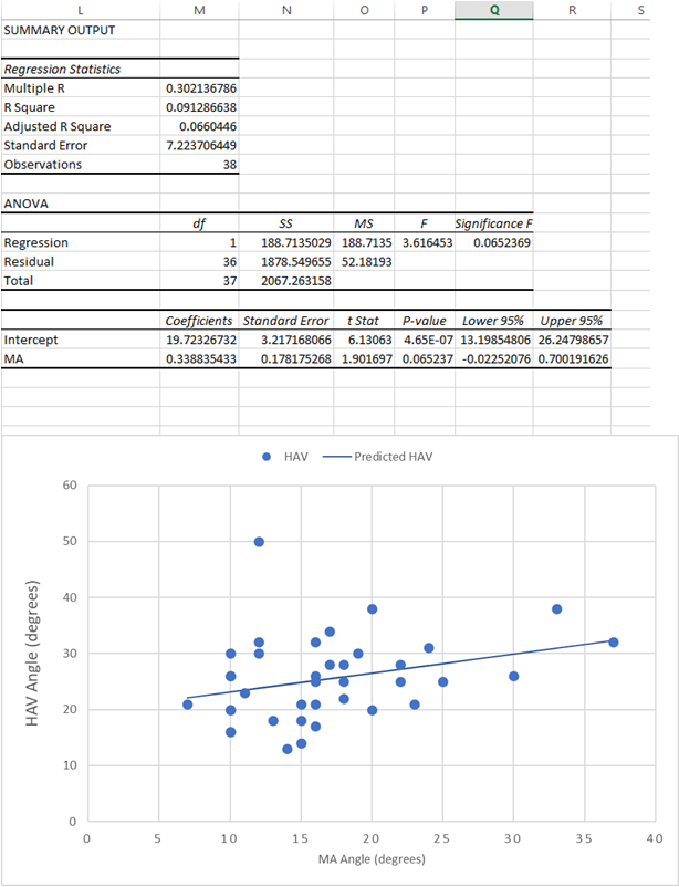
The regressed equation is:

Y = 19.72+0.34x where y is severity of HAV and x is severity of MA.

The regression output indicates value of r at 0.30 and adjusted R² at 0.07 which indicates that there is very weak positive correlation between the factors, MA degree and HAV degree.

The p-value for model as well as p-values for coefficients was also higher than 0.05 indicating that model is not a very good fit.

The scatter plot also indicates weak concentration which is range-bound except for a few outliers.

The residual plot indicates a weak wave-like pattern around x-axis which may indicate that linear regression equation is not appropriate and maybe second order equation will be a better fit.

(b)

The slope of the regression line is given by coefficient of MA, that is 0.34. The standard error is 0.1782. We also see that n = 38. Hence, df = 36.

90% CI can be calculated as: 0.34+- t-stat_c(0.1782)

t-stat is calculated at 36 degrees of freedom and 0.05 tail at either end. From table, this is t = 1.6883

90%CI = 0.34+- (1.6883)(0.1782) = 0.34+-0.30 = 0.64 and 0.04.

Hence, 90% CI ranges from 0.04 to 0.64

(c)

The regressed equation is: Y = 19.72+0.34x where y is severity of HAV and x is severity of MA.

Hence, when x = 30, y = 19.72+0.34(30) = 29.92

Hence, when x = 5, y = 19.72+0.34(5) = 21.42

Despite large change in x-variable, y-variable changes slightly which may lead to questions about the accuracy of the prediction.

Customer Testimonials

Keeping up with college work and assignment dues were impossible! After using the assignment services provided by My Assignment Help, things just got a whole lot easier. Their efficiency in completing my assignments were simply incredible! I recommend this service to anybody facing hardships in finding time to complete their assignments.

Alan, Sydney

In my first year, I was given a ton of paper composing assignments and it got extremely disappointing past a point, as I couldn't concentrate on my additional curricular. This typically influenced me to submit content with less effort and freshness which made me low grades in the end. I became acquainted with about their exposition composing plan and thought that it was practical and from that point forward I've been acing my assignments on Balance Sheet Reconciliations, Thanks to the group.

Ben, Sydney

My finals were nearing and I was very worried as I am somebody with low confidence issues and I needed some proper guidance in terms of internal Assignment and this is exactly when I came across this service aiding website and it helped me tremendously. I felt positive and told them the requirements for my assignment on analyzing Graphs and GDP of two nations and they made it very easy for me to concentrate in m exams and I scored really well. All credits to you guys.

Aaron, New South Wales

Get Help Instantly

Forgot Password Step 1

Forgot Password Step 2

Reset Password

Questions on Introduction to Biostatistics 2020 Assessment 3 Answer

Question 1 [5 marks; 1 mark for each]

Questions 4 [12 marks]

Question 5 [8 marks]

Answer

Customer Testimonials