HI6007 Statistics for Business Decisions Assignment: Tutorial Questions 2 Answer

Assessment Task – Tutorial Questions

Unit Code: HI6007

Unit Name: Statistics for Business Decisions Assignment: Tutorial Questions 2

Weighting: 25%

Purpose: This assignment is designed to assess your level of knowledge of the key topics covered in this unit

Unit Learning Outcomes Assessed:

Students are able to apply appropriate business research methodologies to support decision-making process.
Students are able to identify and apply valid statistical techniques in a given scenario to solve business problems.
Students are able to justify and interpret the results of a statistical analysis in the context of critical reasoning for a business problem solving.
Students are able to apply statistical knowledge to summarize data graphically and statistically, either manually or via a computer package.
Students are able to justify and interpret statistical/analytical scenarios that best fit business solution.
Students are able to justify value and limitations of the statistical techniques to business decision making.

Description: Each week students were provided with three tutorial questions of varying degrees of difficulty. These tutorial questions are available in the Tutorial Folder for each week on Blackboard. The Interactive Tutorials are designed to assist students with the process, skills and knowledge to answer the provided tutorial questions. Your task is to answer a selection of tutorial questions for weeks 7 to 11 inclusive and submit these answers in a single document.

The questions to be answered are;

Week 7

Question 2 (10 marks)

A local health centre noted that in a sample of 400 patients, 80 were referred to them by the local hospital.

Provide a 95% confidence interval for all the patients who are referred to the health centre by the hospital.(5 marks)
What sample size would be required to estimate the proportion of all hospital referrals to the health centre with a margin of error of 0.04 or less at 95% confidence?(5 marks)

Week 8

Question 1 (10 marks)

The average starting salary of students who graduated from colleges of Business in 2009 was $48,400. A sample of 100 graduates of 2010 showed an average starting salary of $50,000. Assume the standard deviation of the population is known to be $8000. We want to determine whether or not there has been a significant increase in the starting salaries.

Step 1. Statement of the hypothesis(1.5 marks)

Step 2. Standardised test statistic formula(1 mark)

Step 3. State the level of significance(1 mark)

Step 4. Decision Rule (Draw a bell to show rejection zone)(3 marks)

Step 5. Calculation of the statistic(2 marks)

Step 6. Conclusion(1.5 marks)

Week 9

Question 3 (10 marks)

The data in the table below presents the hourly quantity of production for three lines of production processes over the first 4 days in XYZ Company. Answer the questions based on the Excel Output given below.

Day	Process 1	Process 2	Process 3
1	33	33	28
2	30	35	36
3	28	30	30
4	29	38	34

ANOVA: Single Factor SUMMARY

Groups	Count	Sum	Average	Variance
Process 1	4	120	30	4.66667
Process 2	4	136	34	11.3333
Process 3	4	128	32	13.3333

ANOVA

Source of Variation	SS	df	MS	F	P value
Between Groups	32	?	?	?
Within Groups	88	?	?
Total	120	11

State the null and alternative hypothesis for single factor ANOVA.(1 mark)
State the decision rule (α = 0.05).(4 marks)
Calculate the test statistic.(3 marks)
Make a decision.(2 marks)

Week 10

Question 2 (10 marks)

Personal wealth tends to increase with age as older individuals have had more opportunities to earn and invest than younger individuals. The following data were obtained from a random sample of eight individuals and records their total wealth (Y) and their current age (X).

Person	Total wealth (‘000s of dollars) Y	Age (Years) X
A	280	36
B	450	72
C	250	48
D	320	51
E	470	80
F	250	40

G	330	55
H

Answer

Q2a)

Total patients (n) = 400

Referred by local hospital (x) = 80

Proportion of those referred by local hospital p = x/n = 80/400 = 0.2

α = 0.5

CI = p ± z score (√p (1-p) / n)

CI = 0.2 ± 1.96 (√0.2 (1-0.2) / 400)

CI = 0.2 ± 1.96 (√0.2*0.8 / 400)

CI = 0.2 ± 1.96 (0.02)

CI = 0.2 ± 0.0392

CI = 0.2392 and 0.1608 or 16.08% to 23.92% of total patients are expected to be refereed by local hospital at 95% CI.

Q2b)

For calculating sample size:

n = z² x p(1-p)/e²

= 1.96² x 0.2(1-0.2)/0.04²

= 3.8416 x 0.2(0.8)/0.0016

= 384.16 or 385

Hence, a sample size of 385 is required to estimate the proportion of all hospital referrals with a margin of error of 0.04 at 95% CI.

Week 8 Q1

Population Mean Salary = $48,400

Sample size = 100, sample mean = $50,000, population SD = $8,000

a) Hypothesis:

H0: µ = 48,000

H1: µ > 48,000

b) One-sample z-test will be used:

z = (ẍ - µ) / (σ/√n)

c) Typically, a significance level of 0.1, 0.05 or 0.01 is used to compare p-value and see whether there is statistical evidence to reject the null hypothesis. Hence, we assume a significance level of α = 0.05.

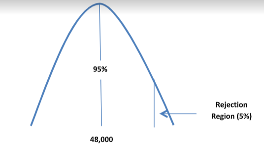
e) Z score is calculated as:

z= (50,000-48,000)/(8000/√100)

z = 2,000/800

z = 2.5

The corresponding p-value at significance level of 0.05 is 0.00621

f) The p-value of 0.00621 is less than the significance level of 0.05 indicating that the result is significant. Hence, we have sufficient statistical evidence to reject the null hypothesis. Hence, we can conclude that there has been a significant increase in the starting salaries.

Week 9 Q3)

a) Hypothesis:

H0: µ1 = µ2 = µ3

H1: At least one mean is different

b) For ANOVA, if F value is greater than F-critical value, then null hypothesis can be rejected. Also, if p-value is less than the significance level of 0.05, then null hypothesis can be rejected.

c) The given data was used to run ANOVA test in excel:

Anova: Single Factor

SUMMARY
Groups	Count	Sum	Average	Variance
Process 1	4	120	30	4.666667
Process 2	4	136	34	11.33333
Process 3	4	128	32	13.33333


ANOVA
Source of Variation	SS	df	MS	F	P-value	F crit
Between Groups	32	2	16	1.636364	0.24766	4.256495
Within Groups	88	9	9.777778

Total	120	11

d) F-value 1.6364 < F critical 4.2565. Also, p-value 0.2477 > significance level of 0.05. Both the results indicate that we do not have sufficient evidence to reject the null hypothesis. Hence, we conclude that there is no significant difference between the mean hourly quantities produced in the three processes.

Week 10 Q2)

a) The estimated regression line is:

y = 45.2159 + 5.3265 x

Where:

y is wealth in ‘000 dollars
x is age in years.

The slope coefficient is the coefficient for independent variable x. In this case, it is 5.3265. This coefficient indicates the amount of change in y for a unit change in x.

b) We know that y = 45.2159 + 5.3265 x

Hence, when x=50:

y = 45.2159 + 5.3265 (50)

y = 45.2159 + 266.325

y = 311.5409

Hence, a 50 year old person is expected to have a wealth of $311,540.9

c) The coefficient of determination is also known as R² and indicates the proportion of variance in the dependent variable (y) that can be explained through independent variable (x). Hence, the amount of change in y that can be attributed to x is coefficient of determination. The value varies from 0 to 1 and higher value indicates a good fit as large proportion of change is being explained by the dependent variable. In this case, R² is 0.91146 or91.146% of change in y can be explained by variable x. This means that the model is a good fit as a very large proportion of variance in wealth is attributed to the dependent variable, age.

i) Hypothesis:

H0: There is no relationship between x and y (slope β = 0)

H1: There is some relationship between x and y (slope β > 0)

ii) t score = (β-0)/SE

iii) The level of significance is 0.1 as given.

iv) If p-value is less than the significance level of 0.1, it indicates that the model is a good fit.

v) z score = (β-0)/SE

= 5.3265-0/0.6777

t score = 7.8597

df = n-1 = 8-1 = 7

Corresponding p-value at df=7 is 0.000051

vi)Since p-value 0.000051 is less than the assumed significance level of α=0.1, we can reject the null hypothesis. Hence, we can conclude that the slope of the regression line is greater than 0 or, there is a positive linear relationship between the variables y and x.

Week 11 Q3)

a) y = 0.0136 + 0.7992 x₁ + 0.2280 x₂ -0.5796 x₃

b)Coefficient of determination R² = 1-(SS_res/SS_tot)

= 1 – (2.6218/(2.6218+45.9634)

= 1- 0.053963

R²= 0.946037

c. Regression df = 3

Error df = 11

Total df = 14

n = 15

SSR = 45.9634

SSE = 2.6218

MSE = SSE/error df = 2.6218/11 = 0.238345

MSR = SSR/regression df = 45.9634/3 = 15.32113

F-ratio = MSR/MSE = 64.28121 Significance F is 0.00000029

Significance F is 0.00000029

At sig level of 0.05, significance F is lower than 0.05 indicating that y is significantly related to the independent variables.

t-stat = Coefficient/SE

The corresponding p-value has been calculated at significance level of 0.05 and a two tailed test was used with df = 14

p-value of 0.5388 > significance level of 0.05 indicating that y is not significantly related to x3.

Customer Testimonials

Keeping up with college work and assignment dues were impossible! After using the assignment services provided by My Assignment Help, things just got a whole lot easier. Their efficiency in completing my assignments were simply incredible! I recommend this service to anybody facing hardships in finding time to complete their assignments.

Alan, Sydney

In my first year, I was given a ton of paper composing assignments and it got extremely disappointing past a point, as I couldn't concentrate on my additional curricular. This typically influenced me to submit content with less effort and freshness which made me low grades in the end. I became acquainted with about their exposition composing plan and thought that it was practical and from that point forward I've been acing my assignments on Balance Sheet Reconciliations, Thanks to the group.

Ben, Sydney

My finals were nearing and I was very worried as I am somebody with low confidence issues and I needed some proper guidance in terms of internal Assignment and this is exactly when I came across this service aiding website and it helped me tremendously. I felt positive and told them the requirements for my assignment on analyzing Graphs and GDP of two nations and they made it very easy for me to concentrate in m exams and I scored really well. All credits to you guys.

Aaron, New South Wales

Get Help Instantly

Forgot Password Step 1

Forgot Password Step 2

Reset Password

HI6007 Statistics for Business Decisions Assignment: Tutorial Questions 2 Answer

Answer

Customer Testimonials