Course: ECO101, Microeconomics

Introduction

Economics is concerned with allocation of scarce resources in the most efficient manner such that benefit is maximized. Hence, the basic premise is that while the human wants are unlimited, the resources available to satisfy these wants are limited. Hence, every human being needs to prioritize the wants and needs so as to draw maximum satisfaction (Mehta, 2007).

The following report discusses the basic microeconomic concepts and how it impacts business activities in an economy. Particularly, the microeconomics concepts related to the calculations and application of production costs will be discussed. This will also cover a discussion on fixed costs and variable costs. Further, the cost structures in a perfect competition market structure will also be discussed.

Types of Costs

There are many concepts related to types of costs, such as, opportunity cost, sunk cost, explicit cost, implicit cost, real cost, money cost, direct cost, indirect cost etc.

However, this report will focus on direct costs and the type of costs that occur while manufacturing a product.

Direct Costs & Indirect Costs

As the name suggests, direct costs refer to the costs that have direct relationship or accountability to the cost of operations. The operations can be manufacturing a product, organizing any process or activity, a service etc. Hence, these costs can be easily accounted for through their relationship with the operations process. They are directly attributed to the process or project in question. Some most common examples include direct material cost, direct labor cost, commissions, wages etc.

On the other hand, indirect costs are those which do not have a direct relationship or accountability to the cost of operations. Hence, these costs are not easily identifiable with the process of operations. For this reason, these costs are also known as non-traceable costs. Some most common examples include accounting expenses, legal expenses, administrative expenses, office rent, security expense, utilities, etc.

However, it must be noted that both direct costs and indirect costs can be fixed or variable. For example, direct material cost is a variable cost but rent for production plant is a fixed cost although both are types of direct costs. Similarly, indirect costs can be variable (for example, hourly-paid administrative job) or fixed (for example, insurance). This concept will be discussed in more detail in following sections (Ahuja, 2012).

Fixed Costs & Variable Costs

As the name suggests, the fixed costs are fixed in nature whether the firm produces 0 quantity or produces 1000 quantity. Hence, for example rent of building will be same whether 0 units are produced or 100 units are produced. The rent has to be paid irrespective of the level of production. Hence, fixed costs don’t change with change in output and they remain unchanged even at 0 level of output. This can be presented graphically as follows (Schiller, 2012):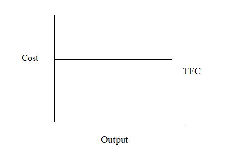

The above graph indicates the total fixed costs (TFC) as a horizontal straight line which is parallel to x-axis where x-axis indicates the level of output. Hence, let’s say the rent of building is $2,000. If the company is producing 0 unit output, the rent will be $2,000 and if the company is producing 100 units output, the rent will still be $2,000. Hence, the straight line parallel to x-axis depicts the phenomenon.

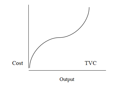
In contrast to fixed costs, variable costs are ‘variable’ in nature with the factor being level of output. Hence with a decline on production level, variable cost declines and with an increase in production level, variable costs also increase. This indicates that when level of output is zero, the variable costs are also zero. Some common examples of variable cost include cost of raw material, labour wages, fuel etc. This can be presented graphically as follows (Schiller, 2012):

Cost TVC

The above graph indicates the total variable costs (TVC) is an upward sloping curve which indicates that as the output, which is represented on x-axis increases, the TVC also increases. Hence, let’s say the raw material cost is $5/unit. If the company is producing 0 unit output, the raw material cost will be $0 and if the company is producing 100 units output, the raw material cost will be $500. Hence, the upward sloping curve depicts the phenomenon.

Total Costs     

It is intuitive to understand that total costs of production are nothing but the sum total of fixed costs and variable costs. In other words, total expenses incurred by a firm in producing a given quantity or commodity is given by following equation:

TC = TFC + TVC

The graph for the above three types of costs can be presented as follows:

In the above graph, the red straight line indicates total fixed costs (TFC) that remains same irrespective of output level. The blue curve represents total variable costs (TVC) that changes with the output level. Hence, it begins at zero and then slopes upwards. The black curve represents total costs (TC) that is sum total of TFC and TVC. It must be observed that the shape of TVC and TC curve is exactly same with the two curves being parallel to each other. Also, the gap between TC and TVC is equal to TFC. This implies that TC increases at a constant rate showing constant returns to the variable factor (Schiller, 2012). 

Average Costs

In simple terms, average is nothing but the division of the sum total by the count of observations. In economics, average cost is calculated by dividing the total cost by number of units. Hence, average cost refers to cost per unit of production. This parameter is widely used for analysis and reports by the management of the company.

Hence, each type of total cost, namely fixed cost, variable costs and total cost itself, can be divided by the units of production so as to get corresponding average cost (Varshney & Maheshwari, 2008):

• Average Fixed Cost (AFC): As discussed, average fixed cost will be calculated by division of total fixed cost by output Q. Hence, AFC = TFC/Q. 

Since TFC is a straight line parallel to x-axis, the AFC curve will be a downward sloping line because the same fixed amount will be distributed over a larger number of units.

• Average Variable Cost (AVC): As discussed, average variable cost will be calculated by division of total variable cost by output Q. Hence, AVC = TVC/Q.

Since TVC is an upward sloping curve, the AVC curve will be a U-shaped curve that is first downward sloping and then it reaches its lowest and then it becomes upward sloping. 

• Average Total Cost (ATC): As discussed, average total cost will be calculated by division of total cost by output Q. Hence, ATC = TC/Q

The graph for the three types of costs, namely Average Fixed Costs (AFC), Average Variable Costs (AVC) and Average Total Costs (ATC) can be presented as follows (Varshney & Maheshwari, 2008):

It can be seen that the red curve is AFC which is downward sloping while blue AVC curve and green ATC curves are U-shaped curves. The U-shaped curves occur because initially, as output increases, the variable cost increases but due to increasing marginal returns, the average variable cost is downward sloping as the variable inputs are more efficient (or productive). However, as more and more units of output are produced, the constant returns set in such that productivity is at a constant rate. At this point, the U-shaped curve is at its lowest. If still more units of output are to be produced, the diminishing marginal returns sets in such that the variable input becomes less efficient or productive in a way that more units of input will be required to produce an extra unit of output. This causes the U-shaped average variable cost curve to slope upwards. The same logic applies to Average Total cost curve also but it lies above AVC curve as ATC also comprises of downward sloping AFC curve (Varshney & Maheshwari, 2008).

Marginal Cost

The marginal cost refers to the additional cost of production that is incurred when one additional unit of output is produced. Hence, MC = TCn- TCn-l

Short Run & Long Run

At this point, it must be differentiated between long run and short run with respect to production. 

In short run, a firm is not as flexible and will be only able to vary the level of variable factors, such as labour, raw material, fuel etc. It cannot change fixed factors, such as plant and equipment. Hence, in short run, a firm will be able to increase or decrease the level of output only by changing the level of variable inputs. Even if demand for product is increasing, it cannot operate at more than its current capacity as it will be unable to add new plants and equipment in short run.

However, in long-run, all the factors become variable. A firm can change level of variable factors as well as fixed factors such as plant size, technology etc. Hence, in long run, a firm can plan and select an optimal combination of inputs and for this reason, long run cost curve is also known as the ‘planning curve’. This can be explained with the following graph (Ahuja, 2012):

Hence, in short run, a firm can select to operate at alternative average cost levels represented by SAC1, SAC2, SAC3, SAC4 or SAC5. This will be determined by the demand level for the product and correspondingly, the firm will opt for a cost curve. 

If a line is drawn through the tangent points of each short run average cost curves, we get the long run average cost (LAC) curve. In other words, the long-run average cost curve is an envelope of the SAC curves.

In the long run, the firm will operate at the most profitable scale of plant. In the above figure, this occurs at point C where the cost is the lowest. Hence, CM is the minimum cost at which the firm can produce OM units which is optimum level of production (Ahuja, 2012). 

Perfect Competition

According to various economists, a market for any product or service can be categorized basis its features as follows: Perfect competition, Monopoly, Monopolistic competition or Oligopoly. 

A perfectly competitive market structure is theoretical in nature and hardly exists in real-life scenarios. However, it is good to understand the concepts of microeconomics in this regard. A perfect competition is characterised by (Debreu, 1972):

1. Many buyers and sellers: A perfect competition market will have a very large number of buyers and sellers. The significance is that this limits any buyer or seller from influencing price or output.
2. Homogenous product: The firms produce output that is exactly identical or homogeneous in nature. Hence, the buyers are indifferent whether they buy products from firm A or firm B as the products are perfect substitutes.
3. Freedom of entry and exit: There are no barriers to entry or exit such that the firms are free to enter or exit at any time.
4. Perfect knowledge of market conditions: Both buyers and sellers have all information related to the market, such as, price, product, technology etc.
5. Uniform price: In a perfect competition market, the product is sold at one single price by all the firms such that no buyer or seller can individually influence the price. For this reason, the seller is also known as the price taker.

The cost/revenue curves of a perfectly competitive firm and industry equilibrium are presented in below graph:

It can be seen in the first figure that the firm has a demand curve which is a horizontal line parallel to the x-axis (representing output). Further, the demand curve is horizontal at equilibrium price P1 as set by the market. 

The demand curve of the firm is also the Average revenue and Marginal revenue curve for the firm. This is because there is uniform price in the market fixed at P1 level. 

The firm will maximize profits at a point where MC=MR. In this case, it will be the point where demand curve and MC intersect. This occurs at the output level Q1.

The similar situation will be presented for each of the firm in the market. However, the cost curves will differ for each firm and will determine whether firm makes profit or incurs losses. Each firm will optimally operate at point where it’s MC=MR.

The second figure presents aggregated position of all the firms in the market. The demand curve will be downward sloping while the supply curve will be upward sloping, resulting in an equilibrium price and output for the industry. The equilibrium price will be same P1 as used by the individual firm in first figure (Debreu, 1972).

Conclusion

The above report discussed various types of cost, particularly fixed cost and variable cost in terms of total cost, average cost and also graphically to understand the shape of various curves.

Further, the report also discussed perfect competition market in terms of the unique characteristics and profit maximization of an individual firm. The report also discussed how market determines equilibrium quantity and price.